I wrote several hundred pages of a book that amounted to exhorting people to alter their own habits of residential energy consumption (turn down the heat, you rogues!), as well as upgrade their built environment (e.g. insulate the attic) and appliances, or even, *gasp*, add solar to their roofs. All this because the numbers, at least in the abstract, showed that such banal acts of conservation (not counting solar) can reduce the carbon footprint of residential energy use by at least 30-50%, from a baseline average of about 12 metric tonnes (1 tonne = 1 metric ton) of CO$_2$-equivalent (CO$_2$e). But a demonstration of how, over the course of roughly 5 years, the net energy use in my house actually fell progressively from around 17,000 kWh of electricity per year down to less than zero (net) seems in order.
I will use this post to emphasize that two-thirds of the total energy reduction, and hence carbon reduction, came from inexpensive or free efficiency/behavioral changes. The last third was then fully offset by a relatively cheap 4.48 kW (<$7,000 after tax incentives) solar system. Thus, efficiency and solar should always be pursued in tandem (in my view), as this reduces overall material and energy use far more effectively than solar alone, and minimizes expenses as well.
Electricity Consumption
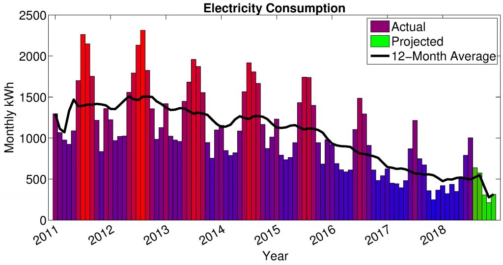
Figure 1. Monthly electricity consumption from January, 2011 through July, 2018, with projected use through 2018 (based upon average energy use in 2017 and relative use in 2018 year-to-date).
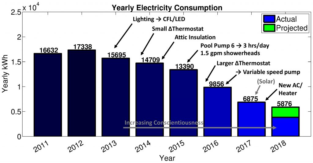
Figure 2. Yearly electricity consumption and approximate timeline of major accompanying efficiency/behavioral changes. Note that solar (added August, 2017) does not affect energy consumption, but is rather a source of energy generation.
Figure 1 shows monthly electricity consumption from January, 2011 through July, 2018 (and projections through the end of 2018), as summarized from previous monthly bills, for my single family house of around 1,500 square feet, with an in-ground swimming pool (the house is all-electric, so no gas, etc. need be added to the monthly energy total). Note that this consumption represents all on-site residential energy use before incorporating any solar generation into our calculations. Given the setting in Mesa, AZ (part of the Phoenix metropolis), it is not at all shocking that there is a cyclical summer peak, with a much smaller winter peak. Now, what accounts for the dramatic drop (about 66%) in energy use over the years (note that both the peaks and baseline consumption fall progressively)? The answer is rather banal, amounting to the following collection of changes (along with approximate time of implementation and my estimate of energy savings):
- High efficiency lighting turnover, i.e. CFLs and LEDs (2012/2013, saving 1,000-1,500 kWh/year)
- Roughly four degree ($^{\circ}$F) change in the thermostat settings: from 78 to 82 $^{\circ}$F in the summer months, and from 70-71 to about 67 $^{\circ}$F in the winter, plus setting the thermostat back when absent (Starting around 2014, becoming more ambitious in 2016; saving 2,000-2,500 kWh/year)
- Blown-in attic insulation (~December 2014, saving additional 500-1,000 kWh/year)
- Single-speed pool pump run-time decreased from 6 hours/day to 3 hours/day (started 2016, saving 1,500 kWh/year)
- Replaced single-speed pool pump with variable speed pump (started 2017, saving an additional 1,000 kWh/year)
- Ultra-low flow shower-heads (1.5 gpm), general reduction in hot water use (started 2015/2016, saving ~1,500-2,000 kWh/year)
- General increase in conscientiousness – turning off TVs, unused appliances, etc. (started 2014/2015, saving 500-1,000 kWh/year)
- New AC/Heat pump in 2017 (saving additional 750-1,000 kWh)
Figure 2 relates yearly energy consumption with the changes above marked, and we see that, in toto, they result in dramatic energy savings, and theory is validated empirically! In fact, such behavioral and efficiency changes were much more important, overall, than solar. Indeed, simply changing the thermostat (free), replacing the lightbulbs (\$100?, \$150?), installing 1.5 gpm showerheads (\$30), and replacing the pool pump with a variable speed pump (\$750) together saved as much as or more energy than the solar system (discussed in a moment). As a brief aside, residential pools are extremely common in the Phoenix area, even in lower-income housing, and a traditional single-speed pool pump usually represents a massive energy drain, sometimes rivaling even the AC. Reducing run-time, or even better, replacing with a variable-speed pump, can reduce this drain by an astounding 90% (see, e.g., this DOE/NREL report)
Solar System and Energy Production

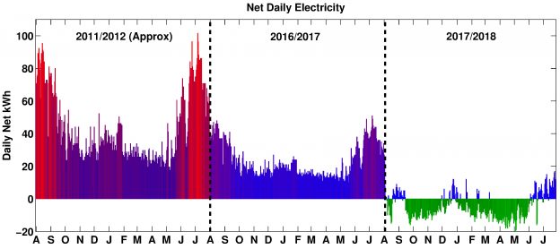
Figure 3. Daily net energy for three year-long intervals. After the installation of solar in August, 2017, a net negative value implies more electricity was produced than was consumed.
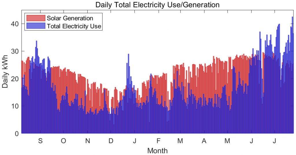
Figure 4. Daily total solar generation and total electricity use since commissioning of the rooftop array almost one year ago (in August, and so the winter months are towards the center of the graph). Most days generation exceeds demand, with peak summer and winter exceptions.
Entering into service on August 3, 2017, our 14-panel, 4.48 kW grid-tie solar system has generated 7,576 kWh at this point, just a few days shy of a single year of operation, and about 1,700 kWh more than the 5,870 kWh consumed in the meantime. Note that this is a grid-tie system, meaning that, during the night and when household demand exceeds solar generation, electricity is drawn from the grid, while when local solar generation exceeds demand, the excess energy is diverted to the grid to be used by other electricity customers. Figure 3 gives daily net energy for yearly intervals before significant conservation (2011/2012, as approximated from later daily energy use data), the year interval before solar (2016/2017), and after solar (2017/2018). Figure 4 shows daily solar generation and total household consumption superimposed on each other.
Now, while the system is net-negative, I still am interested in how much electricity is drawn from the grid, as solar detractors like to point to the fact that grid-tie systems still rely on the grid. Indeed, some go far as to claim that this amounts to solar customers bilking the system and getting a “free ride.” I find this claim absurd on its face, as I still pay a monthly flat fee (one that is appreciably inflated relative to non-solar customers) for the privilege of being connected to the grid, and pay the retail rate for any energy I use. Nevertheless…
Using hourly consumption and generation data available from SRP, in Figure 5 I give an example of a week in late May, showing how during most of the day the local load is covered and excess energy goes to the grid, while at other times there is a load on the grid. Summing hours to days, Figure 6 shows the daily solar energy put on the grid, the daily solar energy consumed locally (i.e. by the house itself), and daily grid energy used.
As can be seen, even if all excess solar energy was lost, the solar system covers roughly half of the local load, and so, even giving zero credit for extra energy production, rooftop solar is highly effective at reducing one’s energy/carbon footprint. In my case, the entire house now only draws about 3,000 kWh from the grid per year, an over 80% reduction from the 2011/2012 baseline.
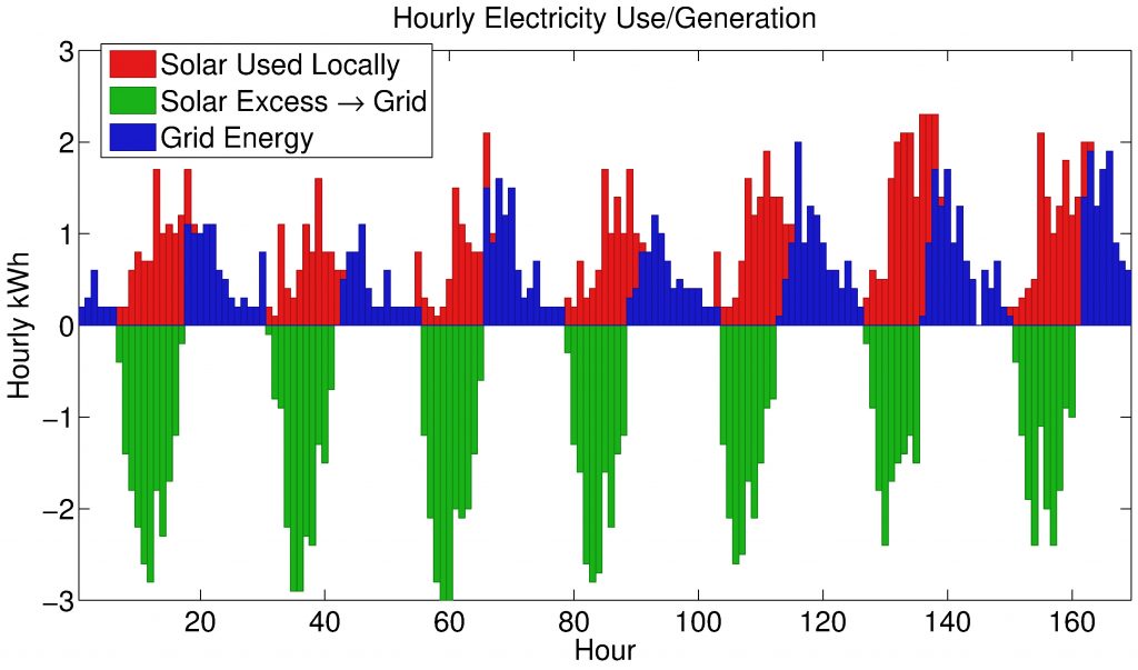
Figure 5. Hourly energy generation and consumption for an example week in late May. The red bars give solar energy that is used locally (i.e. within the house), while the green bars are the extra solar generation that is put onto the grid. Energy drawn from the grid is represented by blue bars (grid energy is mainly used in the evening after the sun is down, but the AC is still needed).
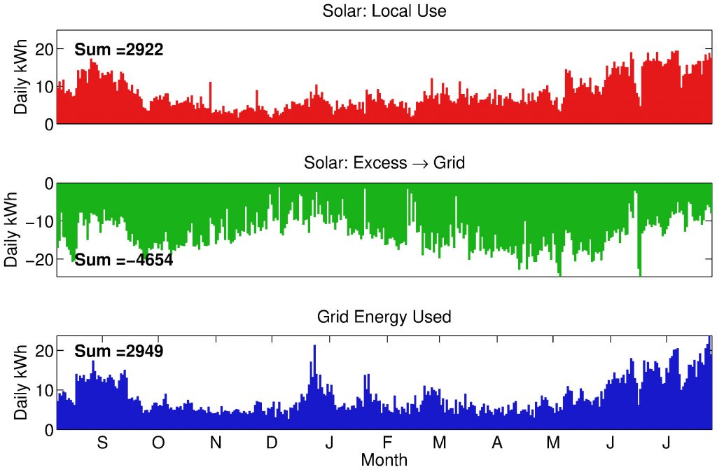
Figure 6. The top series gives daily solar energy used locally, and below is the solar energy put onto the grid. On the bottom is daily grid electricity consumed. Comparing to Figure 3, note how grid energy used at the summer peak has fallen from almost 100 kWh (in 2011/2012) to under 50 kWh with conservation measures, and finally to less than 20 kWh with rooftop solar added to the mix.
Carbon Offset
Finally, I ask how many tonnes of CO$_2$e emissions are avoided via these changes. We could look at grid-average emissions, i.e. average the total CO$_2$e generated from electricity production over all kWh generated, and thus include near-zero carbon sources such as nuclear and hydro. Such a grid-average electricity emissions factor (EF) can be expressed with units kgCO$_2$/kWh, as can all other EFs in this discussion. However, generation from non-fossil sources generally does not change with changes in demand, whereas fossil generation, almost exclusively coal and natural gas, does change seasonally and daily to meet demand. Thus, any marginal change in electricity consumption affects marginal generation, which again, derives almost exclusively from coal and gas.
As we shall see, changes in load preferentially affect gas generation over coal generation, and so, on average in Arizona and using 2017 data, any change in generation has an associated (lifecycle) marginal emissions factor of 0.818 kgCO$_2$/kWh (per kWh delivered, i.e. including transmission and distribution losses), which is less than the EF for all fossil generation, at about 0.961 kgCO$_2$/kWh delivered, but appreciably greater than the (again, lifecycle) grid-average EF of 0.627 kgCO$_2$e/kWh in the AZNM eGRID subregion (for 2016).
It follows that my residence, at negative 1,700 kWh for the year-to-date (just shy of one complete year), has net negative CO$_2$e emissions, at about -1.4 metric tonnes of CO$_2$, based upon the marginal emissions factor. Even using the grid-average, we are net negative by slightly over one tonne CO$_2$e. This is down from around 12 metric tonnes of CO$_2$e in 2012 (using the 2012 edition of eGRID and adjustments as detailed below) on a grid-average basis, or at least 14 metric tonnes of CO$_2$e on a marginal basis (and likely more, given that gas has partially displaced coal in recent years). The derivation of these numbers follows.
Methodology for a marginal emissions factor
We can derive a marginal emissions factor for Arizona, in terms of CO$_2$e/kWh, using hourly power generation and CO$_2$ emissions data from the EPA’s Air Markets Program Data, as previously done by Siler-Evans and colleagues [1]. In a not at all tedious exercise, I have downloaded and processed this data for the AZNM eGRID subregion (the regional grid interconnect expected to provide power for my home), and for Arizona state in particular, using hourly data for all generating units.
Note that SRP, the utility company in my area, is much more reliant on coal than both the AZNM subregion and AZ state average, and derived only about 1.2% of its actual retail electricity from solar in 2017, while 59% of came from coal and 11% from natural gas (note that these figures are higher than the 53% coal and 10% gas reported by SRP, as SRP’s reports included 9.49% of retail electricity demand being met by energy efficiency programs; factoring this out to determine actual generation gives my numbers). Since most SRP generating resources are located in Arizona, and the few out-of-state units are mainly coal-fired (e.g. in Colorado), I consider the Arizona state average marginal emissions rates for power generation to be a minimum for the SRP territory.
Finally, to determine the fossil electricity emissions rates, I factor in upstream natural gas emissions from methane leakage, assumed at 2.4% of gas by mass (the kgCO$_e$/kWh factor for gas generation is then determined for each generating unit using the hourly thermal efficiency), and I also add 13.2 gCO$_2$/kWh(t) for extraction operations. Similarly, coal mine methane and CO$_2$e from mining operations and coal transport are factored into coal emissions based upon the thermal efficiency of each generating unit (details for these calculations are given in the appendix below). From all this, I arrive at a fossil generation emissions rate for each hour of the year (based on year 2017 data).
However, this is still not the marginal emissions factor, which represents the emissions from marginal generating sources that respond to small changes in load. Siler-evans et al. [1] derived the marginal emission factor at time $t$ (MEF$_t$) as
$\text{MEF}_t = \frac{E_{t+1} – E_t}{G_{t+1} – G_t},$
where $E_t$ is the emissions total at time $t$ and $G_t$ is the energy generation total. However, attempting to apply this method to 2017 Arizona data has been problematic for me, as the MEF$_t$ can be very sensitive when generation changes are very small (i.e. dividing anything by a very small number gives a large number). Therefore, I use an alternative “min-max” method, whereby I find the minimum and maximum generation for each 8-hour period of the year, and then determine the marginal emissions rate from the emissions and generation difference at these points. I also calculate the fraction of marginal generation provided by gas versus coal within each 8-hour period.
Arizona fossil generation and emissions rates
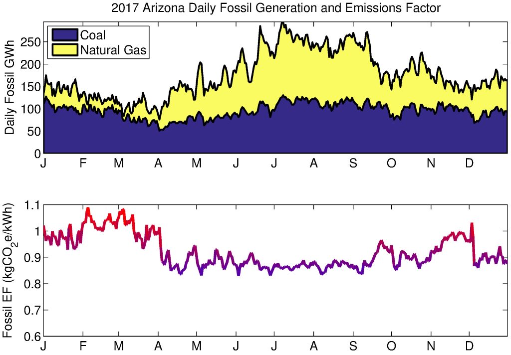
Figure 7. Daily fossil (coal and gas) electricity generation in AZ is plotted on the top panel, while the associated lifecycle emissions factor is given at the bottom (note the bottom plot is scaled to facilitate comparison to the somewhat lower marginal EFs in Figure 8).
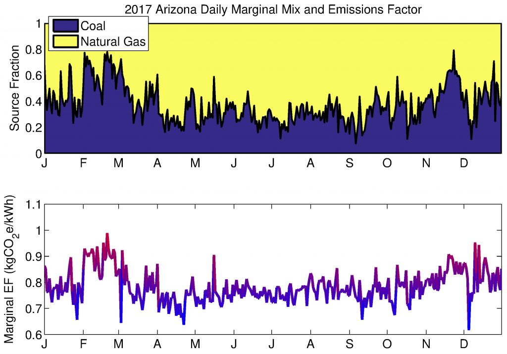
Figure 8. The top panel gives the estimated fractions of marginal electricity generation from coal and gas (note that the fractions must by definition sum to 1). The bottom gives daily marginal EFs for Arizona electricity in 2017. While 54% of all fossil generation was coal in 2017, coal could expected to be the marginal generating source only about 38% of the time (more in winter, less in summer), and so marginal EFs are slightly lower than the average fossil EFs.
Looking at Arizona fossil generation, we see a clear seasonal trend, with increased total energy generation in the summer (for fairly obvious reasons), with most of this increase covered by gas generation. Thus, coal is a smaller fraction of the generating mix in summer (total coal generation is still high in summer). Total fossil generation divided by source, and the lifecycle fossil emissions factor for each day of 2017 is given in Figure 7. Using the method above, I also derive 8-hour marginal emissions factors, and marginal generating mixes. This is shown in Figure 8 on a daily basis. Note that these emissions factors are at the generation level, while there is a small loss of energy involved in power transmission and distribution. Therefore, at the consumption level, I adjust for a 4.23% power loss (average T&D loss in AZNM subregion in 2016, per EPA eGRID).
Now, given hourly solar generation, hourly grid energy consumption, and (approximated from daily) hourly marginal kgCO$_2$e/kWh emissions rates, we can calculate the marginal emissions over the course of the year attributable to my humble, solar-equipped abode. In summary, I calculate:
- Averaged over the year, the lifecycle MEF is 0.784 kgCO$_2$e/kWh at the production level, and 0.818 kgCO$_2$e/kWh at the consumption level (factoring in 4.23% T&D losses).
- The net marginal effect, using hourly solar production and grid-energy consumption data (year-to-date), of my residence is a net negative 1.4 tonnes CO$_2$e, from a net negative 1,700 kWh.
- If we used grid-average EFs for the AZNM subregion, the carbon impact is still net negative by over 1 tonne CO$_2$e.
Note: All figures were created by the author using MATLAB, and may be freely reused with proper attribution to Steffen Eikenberry and a link to this post.
Appendix: Upstream/lifecycle emissions from coal and gas
Following the methodology presented in Chapter 4 of A Fair Share (by the author), I systematically adjust emissions as reported in the 2016 edition of eGIRD for all non-fossil electricity generation for all EPA eGRID subregions to arrive at a grid-average EF of 0.627 kgCO$_2$e/kWh for the AZNM subregion (including 4.23% T&D loss). Chapter 4 is now available for download as supporting material (note that the 2014 edition of eGRID was used in this work: I have updated all numbers to the 2016 edition used here).
Natural gas. Also following Chapter 4, I assume a 2.4% mass leak rate from natural gas systems, appreciably higher than EPA estimates but based upon a large body of literature indicating this is too low (as reviewed in that document), and very similar to the 2.3% leak rate estimated in a new comprehensive assessment just published in Science [2]. I assume 13.2 gCO$_2$/kWh(t) for gas extraction. Calculations also assume a gas density of 0.05 lb/ft$^3$, a heat content of 1,034 Btu/ft$^3$ (per the EIA), and combustion emissions of 0.05444 kgCO$_2$/ft$^3$ (per EPA). I further assume that methane has a 100-year global warming potential of 36 (IPCC AR5 value with climate-carbon feedback). Together, in terms of thermal energy, this yields upstream emissions of 79.5 gCO$_2$e/kWh(t). From EPA AMPD data the thermal efficiency of any operating unit is calculated, and thus total upstream emissions per kWh of electrical energy output are calculated.
As a yearly average, natural gas generation in AZ in 2017 had a thermal efficiency of 44.8%, a direct combustion emission factor of 0.4529 kgCO$_2$/kWh(e), and a lifecycle emissions factor of 0.6305 kgCO$_2$/kWh(e).
Coal. Upstream emissions stem mainly from coal mine methane, mining operations, and coal transport. From the 2016 EIA Coal Report, we have 728.4 million short tons of coal mined in the US (660.8 million metric tons), and 19.78 million Btu / short ton coal in 2017 (EIA). The most recent EPA greenhouse gas inventory gives 2,153 Gg coal mine methane in 2016, and all together these figures yield upstream coal mine emissions of 18.4 gCO$_2$e/kWh(t).
Jamarillo et al. [3] gave coal mining energy for 1997 as 9.081 million barrels of fuel oil, 1.2 billion cubic feet of gas, 34 million gallons of gasoline, and 49.597 billion kWh electricity. I suppose EFs of 12.504 kgCO2e/gallon fuel oil, a gasoline EF of 11.146 kgCO2e/gallon (from Chapter 3 of A Fair Share), and natural gas density, energy content, and upstream emissions as above. For electricity, I set upstream coal emissions to zero as a conservative measure to avoid double-counting, and the method outlined above for grid-average electricity using 2016 EPA eGRID data to give 0.577 kgCO2e/kWh electricity. Dividing among 9.888 billion tonnes of coal mined in 1997 and using a heat content of 23.193 mmBtu/kg finally yields 5 gCO$_2$e/kWh(t).
Also using data reported in Jamarillo et al. suggests an additional 5 gCO$_2$e/kWh(t) for coal transportation. Thus, in sum we get 28.4 gCO$_2$e/kW(t) of upstream coal emissions.
Averaged over the year 2017, in AZ, coal generation had a thermal efficiency of 33.6%, a direct combustion emissions factor of 1.0482 kgCO$_2$e/kW(e), and a lifecycle emissions factor of 1.1328 kgCO$_2$e/kW(e).
Additional references
[1] Siler-Evans, K., Azevedo, I. L., & Morgan, M. G. (2012). Marginal emissions factors for the US electricity system. Environmental science & technology, 46(9), 4742-4748.
[2] Alvarez, R. A., Zavala-Araiza, D., Lyon, D. R., Allen, D. T., Barkley, Z. R., Brandt, A. R., … & Kort, E. A (2018). Assessment of methane emissions from the US oil and gas supply chain. Science, 361(6398), 186-188.
[3] Jaramillo, P., Griffin, W. M., & Matthews, H. S. (2007). Comparative life-cycle air emissions of coal, domestic natural gas, LNG, and SNG for electricity generation. Environmental science & technology, 41(17), 6290-6296.